pysheds
🌎 Simple and fast watershed delineation in python
View the Project on GitHub mdbartos/pysheds
Basic concepts
• Rasters• Views
• File I/O
Hydrologic processing
• DEM conditioning• Flow directions
• Catchment delineation
• Flow accumulation
• Flow distance
• Extracting river networks
• Inundation mapping with HAND
Extract River Network
Preliminaries
The grid.extract_river_network method requires both a catchment grid and an accumulation grid. The catchment grid can be obtained from a flow direction grid, as shown in catchments. The accumulation grid can also be obtained from a flow direction grid, as shown in accumulation.
from pysheds.grid import Grid

# Instantiate grid from raster
grid = Grid.from_raster('./data/dem.tif')
dem = grid.read_raster('./data/dem.tif')

# Resolve flats and compute flow directions
inflated_dem = grid.resolve_flats(dem)
fdir = grid.flowdir(inflated_dem)

# Specify outlet
x, y = -97.294167, 32.73750

# Delineate a catchment
catch = grid.catchment(x=x, y=y, fdir=fdir, xytype='coordinate')

# Clip the view to the catchment
grid.clip_to(catch)

# Compute accumulation
acc = grid.accumulation(fdir, apply_output_mask=False)
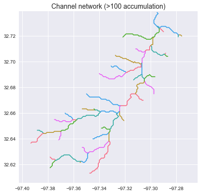
Extracting the river network
To extract the river network at a given accumulation threshold, we can call the grid.extract_river_network method. By default, the method will use an accumulation threshold of 100 cells:
# Extract river network
branches = grid.extract_river_network(fdir, acc > 100)
Plotting code...
import numpy as np
from matplotlib import pyplot as plt
import seaborn as sns

sns.set_palette('husl')
fig, ax = plt.subplots(figsize=(8.5,6.5))

plt.xlim(grid.bbox[0], grid.bbox[2])
plt.ylim(grid.bbox[1], grid.bbox[3])
ax.set_aspect('equal')

for branch in branches['features']:
    line = np.asarray(branch['geometry']['coordinates'])
    plt.plot(line[:, 0], line[:, 1])

_ = plt.title('Channel network (>100 accumulation)', size=14)
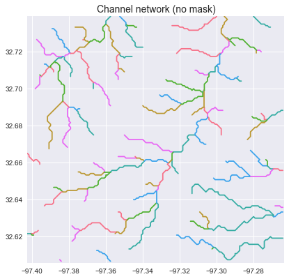
The grid.extract_river_network method returns a dictionary in the geojson format. The branches can be plotted by iterating through the features:
branches = grid.extract_river_network(fdir, acc > 100, apply_output_mask=False)
Plotting code...
sns.set_palette('husl')
fig, ax = plt.subplots(figsize=(8.5,6.5))
plt.xlim(grid.bbox[0], grid.bbox[2])
plt.ylim(grid.bbox[1], grid.bbox[3])
ax.set_aspect('equal')

for branch in branches['features']:
    line = np.asarray(branch['geometry']['coordinates'])
    plt.plot(line[:, 0], line[:, 1])

_ = plt.title('Channel network (no mask)', size=14)
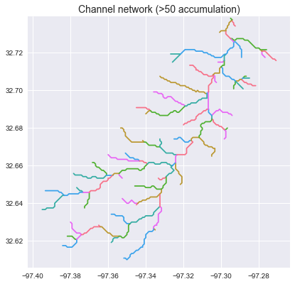
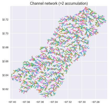
Specifying the accumulation threshold
We can change the geometry of the returned river network by specifying different accumulation thresholds:
branches_50 = grid.extract_river_network(fdir, acc > 50)
branches_2 = grid.extract_river_network(fdir, acc > 2)
Plotting code...
fig, ax = plt.subplots(figsize=(8.5,6.5))

plt.xlim(grid.bbox[0], grid.bbox[2])
plt.ylim(grid.bbox[1], grid.bbox[3])
ax.set_aspect('equal')

for branch in branches_50['features']:
    line = np.asarray(branch['geometry']['coordinates'])
    plt.plot(line[:, 0], line[:, 1])

_ = plt.title('Channel network (>50 accumulation)', size=14)

sns.set_palette('husl')
fig, ax = plt.subplots(figsize=(8.5,6.5))

plt.xlim(grid.bbox[0], grid.bbox[2])
plt.ylim(grid.bbox[1], grid.bbox[3])
ax.set_aspect('equal')

for branch in branches_2['features']:
    line = np.asarray(branch['geometry']['coordinates'])
    plt.plot(line[:, 0], line[:, 1])

_ = plt.title('Channel network (>2 accumulation)', size=14)